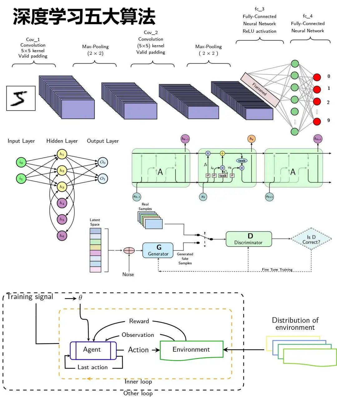
TikZ 复现深度学习五大算法图
本文分享通过 TikZ 绘制深度学习五大算法图,其中深度学习算法内容来源于米酥,以下介绍仅部分算法给出图的完整代码。
全部的源代码打包下载地址为TikZ 复现深度学习五大算法图https://www.latexstudio.net/index/details/index/mid/4132.html。
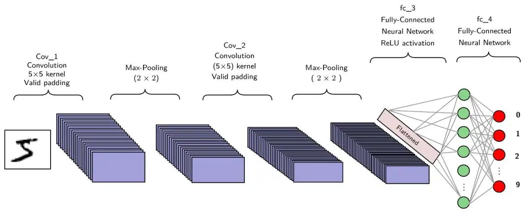
1. 卷积神经网络(CNN)
卷积神经网络(Convolutional Neural Networks, CNN):主要用于图像识别和处理任务,通过卷积层、池化层和全连接层来提取图像特征和进行分类(由于篇幅问题,本文未展示全部代码)。
\documentclass[tikz,border=10pt]{standalone}
\usepackage{ctex,bm,xcolor}
\usetikzlibrary{calc, positioning, arrows.meta, shapes}
\newcommand{\vars}[2]{${\bm#1}_{\bm#2}$}
\usepackage{fontspec}
\usepackage{fontenc}
\setmainfont{Times New Roman}

\tikzset{
......
}

\begin{document}

\begin{tikzpicture}

%%源代码请在链接地址下载

\end{tikzpicture}
\end{document}
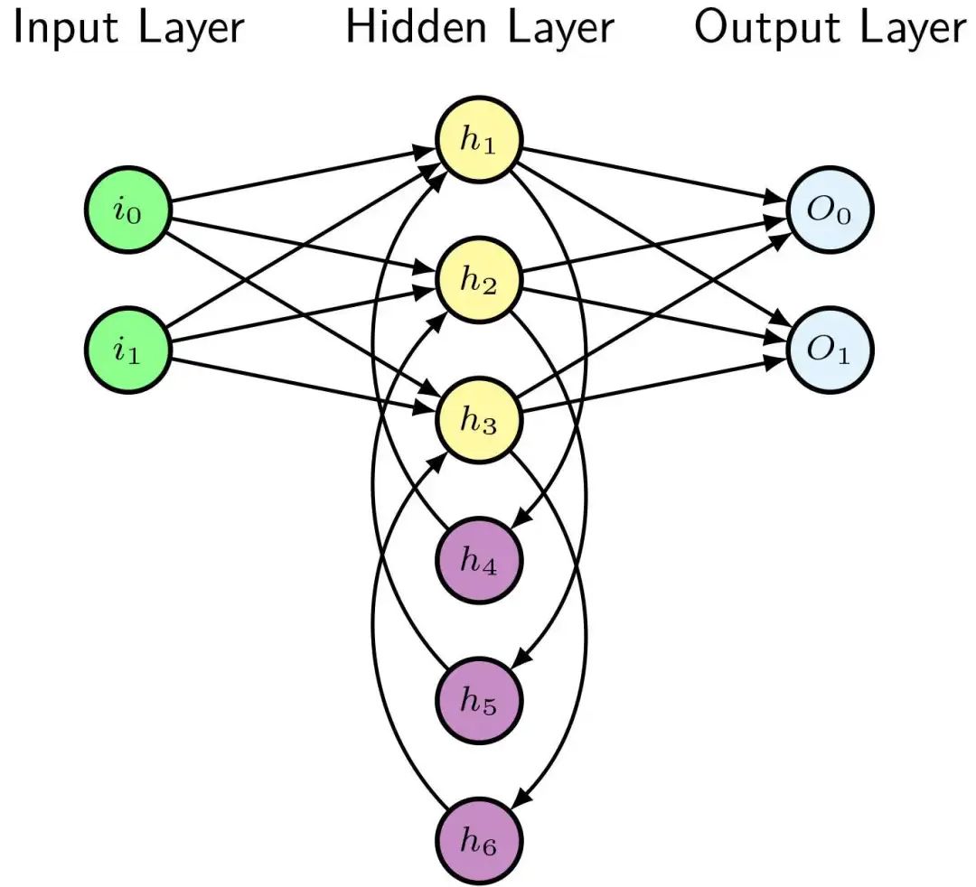
2. 递归神经网络(RNN)
递归神经网络 (Recurrent Neural Networks,RNN):用于处理序列数据,具有记忆能力,可以在自然语言处理、语音识别等领域发挥重要作用(完整代码)。
\documentclass[tikz,border=10pt]{standalone}
\usepackage{tikz-network}
\usetikzlibrary{calc, positioning, arrows.meta, shapes}
\usepackage{fontspec}
\usepackage{fontenc}
\setmainfont{Times New Roman}

\begin{document}
\sffamily
\begin{tikzpicture}
\Vertex[label=$i_1$,style={line width=1pt,fill=green!45}]{A1}
\Vertex[y=1,label=$i_0$,style={line width=1pt,fill=green!45}]{A2}

\foreach \y/\n in {1.5/1,0.5/2,-0.5/3}{
\Vertex[y=\y,x=2.5,label=$h_\n$,style={line width=1pt,fill=yellow!45}]{B\n}
}

\foreach \y/\n in {-1.5/4,-2.5/5,-3.5/6}{
\Vertex[y=\y,x=2.5,label=$h_\n$,style={line width=1pt,fill=violet!45}]{B\n}
}

\Vertex[x=5,label=$O_1$,style={line width=1pt,fill=cyan!15}]{C1}
\Vertex[x=5,y=1,label=$O_0$,style={line width=1pt,fill=cyan!15}]{C2}

\foreach \i in {1,2}{
\foreach \n in {1,2,3}{
\Edge[Direct,style={line width=0.75pt,black}](A\i)(B\n)
}}

\foreach \i in {1,2,3}{
\foreach \n in {1,2}{
\Edge[Direct,style={line width=0.75pt,black}](B\i)(C\n)
}}

\Edge[Direct,style={line width=0.75pt,black},bend=45](B4)(B1)
\Edge[Direct,style={line width=0.75pt,black},bend=45](B5)(B2)
\Edge[Direct,style={line width=0.75pt,black},bend=45](B6)(B3)

\Edge[Direct,style={line width=0.75pt,black},bend=45](B1)(B4)
\Edge[Direct,style={line width=0.75pt,black},bend=45](B2)(B5)
\Edge[Direct,style={line width=0.75pt,black},bend=45](B3)(B6)

\node[above=1cm] at (A2){Input Layer};
\node[above=0.5cm] at (B1){Hidden Layer};
\node[above=1cm] at (C2){Output Layer};

\end{tikzpicture}
\end{document}
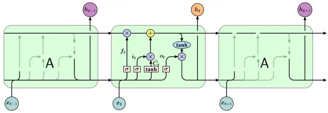
3. 长短期记忆网络(LSTM)
长短期记忆网络 (Long Short-Term Memory,LSTM):RNN 的一种特殊形式,用于解决传统 RNN 在处理长序列数据时出现的梯度消失或梯度爆炸的问题,适用于时间序列预测等任务(完整代码)。
\documentclass[tikz,border=10pt]{standalone}
\usepackage{ctex,bm,xcolor}
\usetikzlibrary{calc, positioning, arrows.meta, shapes}
\newcommand{\vars}[2]{${\bm#1}_{\bm#2}$}
\usepackage{fontspec}
\usepackage{fontenc}
\setmainfont{Times New Roman}
\tikzset{
myfont/.style={
font=\footnotesize\sffamily
},
frame/.style={
rectangle,
rounded corners=5mm,
draw,gray,
fill=green!15!white,
very thick,
},
add/.style={
circle,
draw, thick,
fill=yellow!60,
inner sep=.5pt,
minimum height =3mm,
},
prod/.style={
circle,
draw, thick,
fill=lightgray!40!blue!30,
inner sep=.5pt,
minimum height =3mm,
},
function/.style={
ellipse,
draw, thick,
fill=cyan!30,
inner sep=1pt
},
cell/.style={
circle,draw,fill=magenta!30,
line width = .75pt,
minimum width=8mm,
inner sep=1pt,
},
hidden/.style={
circle,draw,fill=orange!50,
line width = .75pt,
minimum width=8mm,
inner sep=1pt,
},
input/.style={
circle,draw,
fill=teal!30,
line width = .75pt,
minimum width=8mm,
inner sep=1pt,
},
actfunc/.style={
rectangle, draw,
fill=pink!30,
minimum width=4.25mm,
minimum height=3.75mm,
inner sep=1pt,
thick,
},
ArrowC1/.style={
rounded corners=2mm,
>=Stealth[round],
very thick,
},
ArrowC2/.style={
rounded corners=3mm,
>=Stealth[round],
very thick,
}
}
\begin{document}
\begin{tikzpicture}
%%% First ===========================================
\begin{scope}[xshift=0em,yshift=0em]
\node [frame, minimum height =4cm, minimum width=6cm] at (0,0) {};
\node (ibox1) at (-2,-0.8) {};
\node (ibox2) at (-1.35,-0.8) {};
\node (ibox3) at (-0.45,-0.8) {};
\node (ibox4) at (0.5,-0.8) {};
\node (mux1) at (-2,1.5) {};
\node (add1) at (-0.5,1.5) {};
\node (mux2) at (-0.5,0) {};
\node (mux3) at (1.5,0) {};
\node (func1) at (1.5,0.75) {};
\node(c) at (-3.1,1.5) {};
\node(h) at (-3.1,-1.5) {};
\node[input] (x) at (-2.5,-3) {\vars{x}{t-1}};
\node (c2) at (4,1.5) {};
\node (h2) at (4,-1.5) {};
\node[hidden,fill=violet!45] (x2) at (2.5,3) {\vars{h}{t-1}};
\draw [->, ArrowC1] (c) -- (mux1) -- (add1) -- (c2);
\draw [opacity=0.3,ArrowC2] (h) -| (ibox4);
\draw [opacity=0.3,ArrowC1] (h) -| (ibox1);
\draw [opacity=0.3,ArrowC1] (h) -| (ibox2);
\draw [opacity=0.3,ArrowC1] (h) -| (ibox3);
\draw [ArrowC1] (x) -- (x |- h) -| (ibox1);
\draw [->, opacity=0.3,ArrowC2] (ibox1) -- (mux1);
\node [right=1.5pt] () at ($(ibox1)!.5!(mux1)$) {};
\draw [->,opacity=0.3, ArrowC2] (ibox2) |- (mux2);
\node [right=2pt] () at (ibox2 |- mux2) {};
\draw [->, opacity=0.3,ArrowC2] (ibox3) -- (mux2);
\node [label=right:{\sffamily\Huge A}, left=.5pt] () at ($(ibox3)!.5!(mux2)$) {};
\draw [->,opacity=0.3, ArrowC2] (ibox4) |- (mux3);
\node [right=2pt] () at (ibox4 |- mux3) {};
\draw [->,opacity=0.3, ArrowC2] (mux2) -- (add1);
\draw [->, opacity=0.3,ArrowC1] (add1) -| (func1);
\draw [->,opacity=0.3, ArrowC2] (func1) -- (mux3);
\draw [->, ArrowC2] (mux3) |- (h2);
\draw (c2 -| x2) ++(0,-0.15) coordinate (i1);
\draw [-, ArrowC2] (h2 -| x2) -| (i1);
\draw [->, ArrowC2] (i1)++(0,0.3) -- (x2);
\end{scope}
%%% Second ===========================================
\begin{scope}[xshift=18.5em,yshift=0em]
\node [frame, minimum height =4cm, minimum width=6cm] at (0,0) {};
\node [actfunc] (ibox1) at (-2,-0.8) {$\bm\sigma$};
\node [actfunc] (ibox2) at (-1.35,-0.8) {$\bm\sigma$};
\node [actfunc, minimum width=9mm] (ibox3) at (-0.45,-0.8) {$\bm\tanh$};
\node [actfunc] (ibox4) at (0.5,-0.8) {$\bm\sigma$};
\node [prod] (mux1) at (-2,1.5) {$\bm\times$};
\node [add] (add1) at (-0.5,1.5) {$\bm+$};
\node [prod] (mux2) at (-0.5,0) {$\bm\times$};
\node [prod] (mux3) at (1.5,0) {$\bm\times$};
\node [function] (func1) at (1.5,0.75) {$\bm\tanh$};
% \node[cell] (c) at (-4,1.5) {\vars{c}{t-1}};
% \node[hidden] (h) at (-4,-1.5) {\vars{h}{t-1}};
\node[input] (x) at (-2.5,-3) {\vars{x}{t}};
\node (c2) at (4,1.5) {};
\node(h2) at (4,-1.5) {};
\node[hidden] (x2) at (2.5,3) {\vars{h}{t}};
\draw [->, ArrowC1] (c) -- (mux1) -- (add1) -- (c2);
\draw [ArrowC2] (h) -| (ibox4);
\draw [ArrowC1] (h) -| (ibox1);
\draw [ArrowC1] (h) -| (ibox2);
\draw [ArrowC1] (h) -| (ibox3);
\draw [ArrowC1] (x) -- (x |- h) -| (ibox1);
\draw [->, ArrowC2] (ibox1) -- (mux1);
\node [label=left:$\bm{f_t}$,right=1.5pt] () at ($(ibox1)!.5!(mux1)$) {};
\draw [->, ArrowC2] (ibox2) |- (mux2);
\node [label=left:$\bm{i_t}$, right=2pt] () at (ibox2 |- mux2) {};
\draw [->, ArrowC2] (ibox3) -- (mux2);
\node [label=right:$\bm{\tilde{C}_t}$, left=.5pt] () at ($(ibox3)!.5!(mux2)$) {};
\draw [->, ArrowC2] (ibox4) |- (mux3);
\node [label=left:$\bm{o_t}$, right=2pt] () at (ibox4 |- mux3) {};
\draw [->, ArrowC2] (mux2) -- (add1);
\draw [->, ArrowC1] (add1) -| (func1);
\draw [->, ArrowC2] (func1) -- (mux3);
\draw [->, ArrowC2] (mux3) |- (h2);
\draw (c2 -| x2) ++(0,-0.15) coordinate (i1);
\draw [-, ArrowC2] (h2 -| x2) -| (i1);
\draw [->, ArrowC2] (i1)++(0,0.3) -- (x2);
\end{scope}
%%% third ===========================================
\begin{scope}[xshift=37em,yshift=0em]
\node [frame, minimum height =4cm, minimum width=6cm] at (0,0) {};
\node (ibox1) at (-2,-0.8) {};
\node (ibox2) at (-1.35,-0.8) {};
\node (ibox3) at (-0.45,-0.8) {};
\node (ibox4) at (0.5,-0.8) {};
\node (mux1) at (-2,1.5) {};
\node (add1) at (-0.5,1.5) {};
\node (mux2) at (-0.5,0) {};
\node (mux3) at (1.5,0) {};
\node (func1) at (1.5,0.75) {};
\node(c) at (-3.1,1.5) {};
\node(h) at (-3.1,-1.5) {};
\node[input] (x) at (-2.5,-3) {\vars{x}{t+1}};
\node (c2) at (4,1.5) {};
\node (h2) at (4,-1.5) {};
\node[hidden,fill=violet!45] (x2) at (2.5,3) {\vars{h}{t+1}};
\draw [->, ArrowC1] (c) -- (mux1) -- (add1) -- (c2);
\draw [opacity=0.3,ArrowC2] (h) -| (ibox4);
\draw [opacity=0.3,ArrowC1] (h) -| (ibox1);
\draw [opacity=0.3,ArrowC1] (h) -| (ibox2);
\draw [opacity=0.3,ArrowC1] (h) -| (ibox3);
\draw [ArrowC1] (x) -- (x |- h) -| (ibox1);
\draw [->, opacity=0.3,ArrowC2] (ibox1) -- (mux1);
\node [right=1.5pt] () at ($(ibox1)!.5!(mux1)$) {};
\draw [->,opacity=0.3, ArrowC2] (ibox2) |- (mux2);
\node [right=2pt] () at (ibox2 |- mux2) {};
\draw [->, opacity=0.3,ArrowC2] (ibox3) -- (mux2);
\node [label=right:{\sffamily\Huge A}, left=.5pt] () at ($(ibox3)!.5!(mux2)$) {};
\draw [->,opacity=0.3, ArrowC2] (ibox4) |- (mux3);
\node [right=2pt] () at (ibox4 |- mux3) {};
\draw [->,opacity=0.3, ArrowC2] (mux2) -- (add1);
\draw [->, opacity=0.3,ArrowC1] (add1) -| (func1);
\draw [->,opacity=0.3, ArrowC2] (func1) -- (mux3);
\draw [->, ArrowC2] (mux3) |- (h2);
\draw (c2 -| x2) ++(0,-0.15) coordinate (i1);
\draw [-, ArrowC2] (h2 -| x2) -| (i1);
\draw [->, ArrowC2] (i1)++(0,0.3) -- (x2);
\end{scope}
\end{tikzpicture}
\end{document}
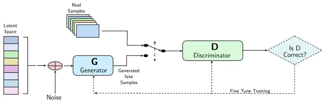
4. 生成对抗网络(GAN)
生成对抗网络 (Generative Adversarial Networks, GAN):由生成器和判别器组成的框架,用于生成逼真的样本数据,被广泛应用于图像生成、视频生成等领域(源代码请到网站下载)。
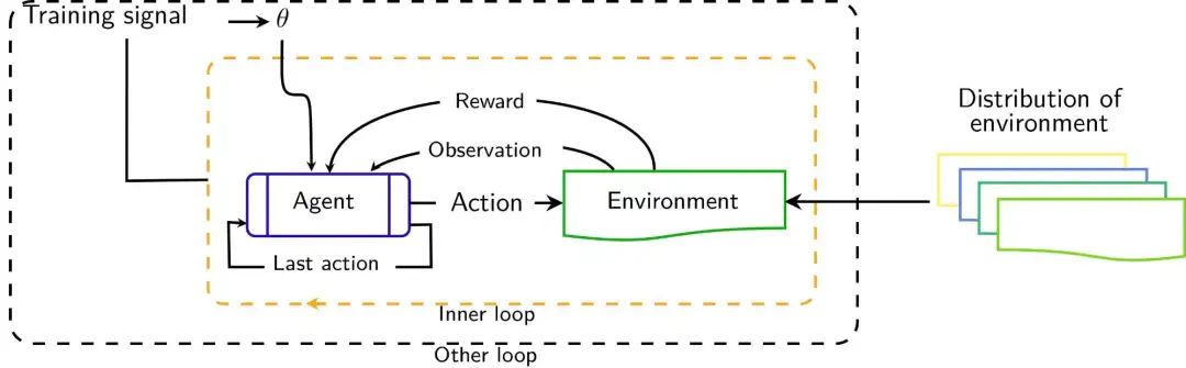
5. 强化学习(RL)
强化学习 (Reinforcement Learning, RL):以智能体与环境的交互来达到特定目标的一种机器学习方式。其中,深度 Q 网络 (Deep Q-Network.DQN)是一种融合深度学习和强化学习的方法,被用于解决复杂的決策问题(源代码请到网站下载)。
最后,感谢大家的支持和关注!
入门资料,免费知识代码:
https://flowus.cn/latex/share/66110e84-b24a-4cd5-b8a7-2ba2afb35a30
精心制作免费视频教程:
https://space.bilibili.com/209746320