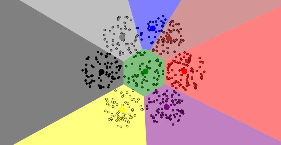
在数据分析和机器学习领域,聚类作为一种核心技术,对于从未标记数据中发现模式和洞察力至关重要。聚类的过程是将数据点分组,使得同组内的数据点比不同组的数据点更相似,这在市场细分到社交网络分析的各种应用中都非常重要。然而,聚类最具挑战性的方面之一在于确定最佳聚类数,这一决策对分析质量有着重要影响。
虽然大多数数据科学家依赖肘部图和树状图来确定K均值和层次聚类的最佳聚类数,但还有一组其他的聚类验证技术可以用来选择最佳的组数(聚类数)。我们将在sklearn.datasets.load_wine问题上使用K均值和层次聚类来实现一组聚类验证指标。以下的大多数代码片段都是可重用的,可以在任何数据集上使用Python实现。
接下来我们主要介绍以下主要指标:
Gap统计量(Gap Statistics)(!pip install --upgrade gap-stat[rust])
Calinski-Harabasz指数(Calinski-Harabasz Index )(!pip install yellowbrick)
Davies Bouldin评分(Davies Bouldin Score )(作为Scikit-Learn的一部分提供)
轮廓评分(Silhouette Score )(!pip install yellowbrick)
引入包和加载数据
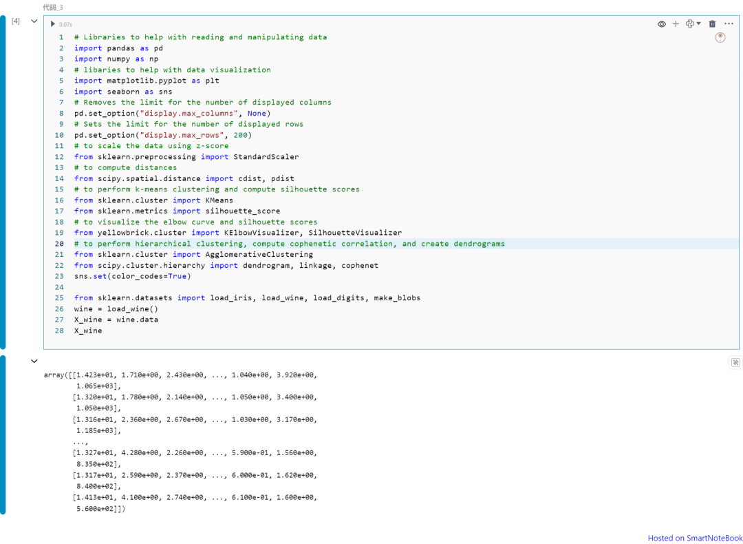
import pandas as pdimport numpy as npimport matplotlib.pyplot as pltimport seaborn as snspd.set_option("display.max_columns", None)pd.set_option("display.max_rows", 200)from sklearn.preprocessing import StandardScalerfrom scipy.spatial.distance import cdist, pdistfrom sklearn.cluster import KMeansfrom sklearn.metrics import silhouette_scorefrom yellowbrick.cluster import KElbowVisualizer, SilhouetteVisualizerfrom sklearn.cluster import AgglomerativeClusteringfrom scipy.cluster.hierarchy import dendrogram, linkage, cophenetsns.set(color_codes=True)
from sklearn.datasets import load_iris, load_wine, load_digits, make_blobswine = load_wine()X_wine = wine.dataX_wine
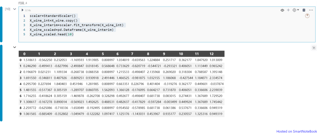
标准化数据:
scaler=StandardScaler()X_wine_int=X_wine.copy()X_wine_interim=scaler.fit_transform(X_wine_int)X_wine_scaled=pd.DataFrame(X_wine_interim)X_wine_scaled.head(10)
Gap统计量(Gap Statistics)

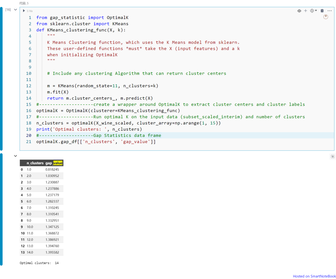
from gap_statistic import OptimalKfrom sklearn.cluster import KMeansdef KMeans_clustering_func(X, k):
""" K Means Clustering function, which uses the K Means model from sklearn. These user-defined functions *must* take the X (input features) and a k when initializing OptimalK """ m = KMeans(random_state=11, n_clusters=k) m.fit(X) return m.cluster_centers_, m.predict(X)optimalK = OptimalK(clusterer=KMeans_clustering_func)n_clusters = optimalK(X_wine_scaled, cluster_array=np.arange(1, 15))print('Optimal clusters: ', n_clusters)optimalK.gap_df[['n_clusters', 'gap_value']]
plt.figure(figsize=(10,6))n_clusters=3plt.plot(optimalK.gap_df.n_clusters.values, optimalK.gap_df.gap_value.values, linewidth=2)plt.scatter(optimalK.gap_df[optimalK.gap_df.n_clusters == n_clusters].n_clusters, optimalK.gap_df[optimalK.gap_df.n_clusters == n_clusters].gap_value, s=250, c='r')plt.grid(True)plt.xlabel('Cluster Count')plt.ylabel('Gap Value')plt.title('Gap Values by Cluster Count')plt.axvline(3, linestyle="--")plt.show()
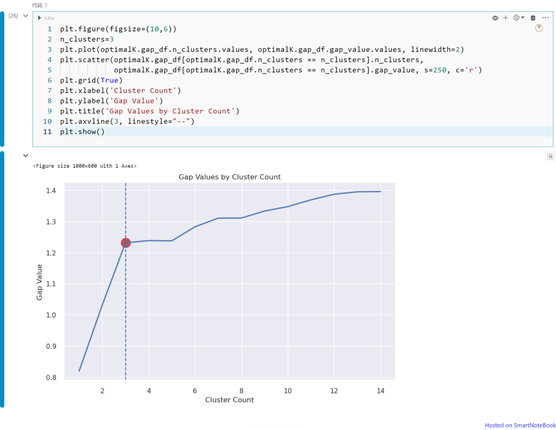
上图展示不同K值(从K=1到14)下的Gap统计量值。请注意,在本例中我们可以将K=3视为最佳的聚类数。如上所述,可以从图中获得Gap统计量的拐点。
Calinski-Harabasz指数(Calinski-Harabasz Inde)
Calinski-Harabasz指数,也称为方差比准则,是所有组的组间距离与组内距离之和(群内距离)的比值。较高的分数表示更好的聚类紧密度。可以使用Python的YellowBrick库中的KElbow visualizer来计算。
plt.figure(figsize=(10,6))model = KMeans(random_state=1)visualizer = KElbowVisualizer( model, k=(2, 10), metric="calinski_harabasz", timings=True)visualizer.fit(X_wine_scaled) visualizer.show()
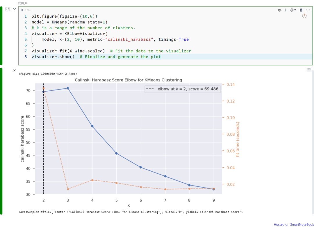
上图展示不同K值(从K=1到9)下的Calinski Harabasz指数。请注意,在本例中我们可以将K=2视为最佳的聚类数。如上所述,可以从图中获得Calinski Harabasz指数的最大值。
使用“metric”超参数选择用于评估群组的评分指标。默认使用的指标是均方失真,定义为每个点到其最近质心(即聚类中心)的距离平方和。其他一些指标包括:
distortion:点到其聚类中心的距离平方和的均值
silhouette:聚类内距离与数据点到其最近聚类中心距离的比率,对所有数据点求平均
calinski_harabasz:群内到群间离散度的比率
Davies-Bouldin指数(Davies-Bouldin Index)
Davies-Bouldin指数计算为每个聚类(例如Ci)与其最相似聚类(例如Cj)的平均相似度。这个指数表示聚类的平均“相似度”,其中相似度是一种将聚类距离与聚类大小相关联的度量。具有较低Davies-Bouldin指数的模型在聚类之间有更好的分离效果。对于聚类i到其最近的聚类j的相似度R定义为(Si + Sj) / Dij,其中Si是聚类i中每个点到其质心的平均距离,Dij是聚类i和j质心之间的距离。一旦计算了相似度(例如i = 1, 2, 3, ..., k)到j,我们取R的最大值,然后按聚类数k进行平均。
from sklearn.metrics import davies_bouldin_scoredef get_Hmeans_score( data, distance, link, center): """ returns the score regarding Davies Bouldin for points to centers INPUT: data - the dataset you want to fit Agglomerative to distance - the distance for AgglomerativeClustering link - the linkage method for AgglomerativeClustering center - the number of clusters you want (the k value) OUTPUT:
score - the Davies Bouldin score for the Hierarchical model fit to the data """ hmeans = AgglomerativeClustering(n_clusters=center,linkage=link) model = hmeans.fit_predict(data) score = davies_bouldin_score(data, model) return score
centers = list(range(2, 10)) avg_scores = []for center in centers: avg_scores.append(get_Hmeans_score(X_wine_scaled, "euclidean", "average", center))plt.figure(figsize=(15,6)); plt.plot(centers, avg_scores, linestyle="-", marker="o", color="b")plt.xlabel("K")plt.ylabel("Davies Bouldin score")plt.title("Davies Bouldin score vs. K")
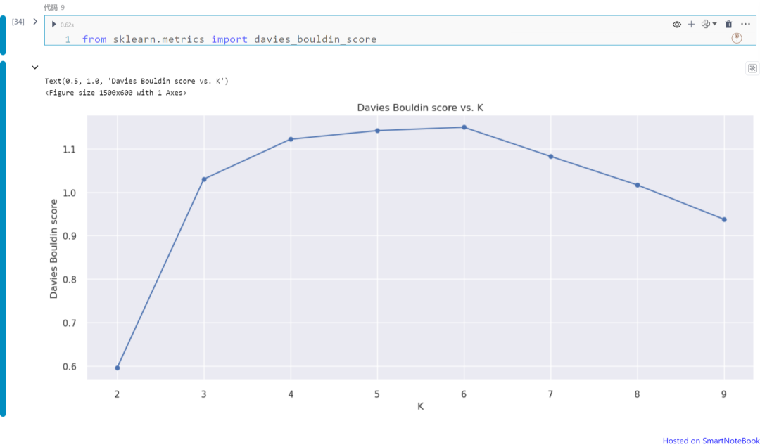
上图展示不同K值(从K=1到9)下的Davies Bouldin指数。请注意,在本例中我们可以将K=2视为最佳的聚类数。如上所述,可以从图中获得Davies Bouldin指数的最小值,该值对应于最优化的聚类数。
轮廓分数(Silhouette Score)
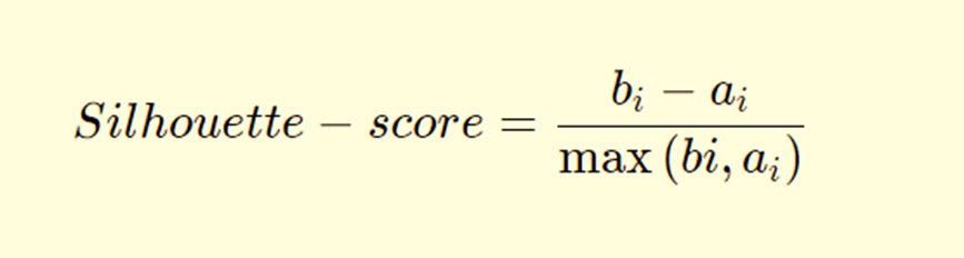
轮廓分数衡量了考虑到聚类内部(within)和聚类间(between)距离的聚类之间的差异性。在下面的公式中,bi代表了点i到所有不属于其所在聚类的任何其他聚类中所有点的平均最短距离;ai是所有数据点到其聚类中心的平均距离。如果bi大于ai,则表示该点与其相邻聚类分离良好,但与其聚类内的所有点更接近。
plt.figure(figsize=(10,6))model = KMeans(random_state=1)visualizer = KElbowVisualizer( model, k=(2, 10), metric="silhouette", timings=True)visualizer.fit(X_wine_scaled) visualizer.show()
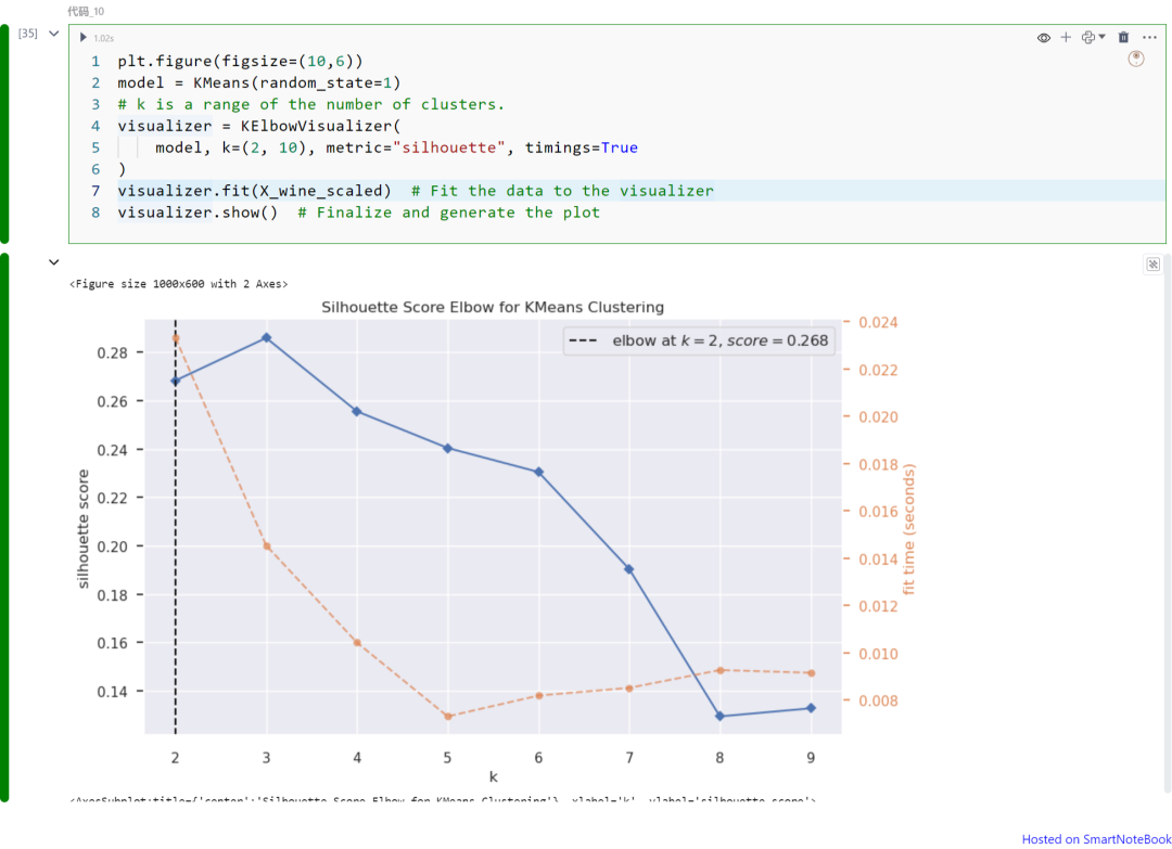
上图展示不同K值(从K=1到9)下的轮廓分数。请注意,在本例中我们可以将K=2视为最佳的聚类数。如上所述,轮廓分数可以从图中获得最大值,该值对应于最优化的聚类数。
在数据分析和机器学习中,聚类是一项关键技术,帮助我们从未标记的数据中发现模式和洞察。确定最佳聚类数是聚类过程中的重要挑战,影响分析质量。本文介绍了多种聚类验证技术如Gap统计量、Calinski-Harabasz指数、Davies Bouldin指数和轮廓分数,这些指标可以帮助我们选择最优化的聚类数,提升聚类结果的有效性和可靠性。


